To forecast storms accurately, you’ll need to layer multiple data streams into one coherent picture. Start with surface observations and upper-air soundings to validate the current atmospheric state. Map upper-level troughs, jet streaks, and shortwaves early, then cross-check model output against real-time observations to catch biases. Read instability, moisture, and wind shear together as a system. Use radar and satellite for precise timing. The seven tips ahead break down exactly how to do this.
Key Takeaways
- Prioritize surface observations and upper-air soundings to validate atmospheric conditions before trusting model outputs for storm forecasting.
- Track large-scale patterns like 500 mb troughs and jet streaks 5–7 days out, narrowing focus as storms approach.
- Cross-check GFS and ECMWF model outputs against real-time observations to identify biases and improve forecast accuracy.
- Transition from synoptic to nowcasting analysis within 6 hours, using radar, satellite, and lightning data for precision.
- Recognize local triggers like surface boundaries, terrain features, and differential heating as key convection initiation factors.
Start Every Weather Forecast With the Current Atmospheric State
Before you examine model guidance or long-range outlooks, anchor your forecast in what the atmosphere is actually doing right now. Surface observations give you immediate temperature, humidity, wind, and pressure data that reveal whether storm development is viable. Don’t skip this step — models inherit errors when initial conditions are misread.
Before the models, before the outlooks — read what the atmosphere is doing right now.
Vertical profiling through upper-air soundings adds critical structure, exposing instability layers, moisture depth, and wind behavior across standard pressure levels like 500 mb, 700 mb, and 850 mb. These profiles tell you how the atmosphere is organized from the ground up.
Layer in climatology patterns to determine whether current conditions deviate from historical norms. That deviation often signals elevated severe-weather potential.
Ground your forecast in observed reality first — everything else builds from there.
Time Your Forecast Window From Days Out to Nowcasting
When a potential storm system appears on global models like the ECMWF or GFS 5–7 days out, you should begin tracking large-scale pattern indicators such as 500 mb trough positions, jet streak alignments, and ensemble spread.
As the event window narrows to 24–48 hours, shift your focus to mesoscale features—surface boundaries, low-level jet activity, and sounding-derived instability indices.
Within 6 hours of impact, switch fully to nowcasting mode, integrating real-time radar loops, GOES satellite imagery, and lightning detection data to refine storm timing and intensity.
Start Monitoring Days Ahead
Effective storm forecasting starts days before the first raindrop falls. At the 5–7 day range, you’re working with global models like ECMWF and GFS to identify broad severe-weather setups. Monitor long-wave troughs at 500 mb and track jet streaks that signal enhanced lift regions.
Climate variability influences background atmospheric states, so compare current patterns against climatological baselines to detect anomalies early.
As you move inside 72 hours, refine your analysis using ensemble guidance to assess forecast consensus and uncertainty. Flag aviation hazards by identifying developing convective corridors, icing levels, and turbulence zones within model output.
Cross-check NWP solutions against current upper-air soundings to catch model drift. Early monitoring gives you the lead time needed to communicate probabilistic storm threats accurately and confidently.
Narrow Focus Near Impact
As the storm window closes to 24–48 hours, shift your attention from synoptic-scale pattern recognition to mesoscale feature analysis. Track surface boundaries, monitor radar loops for developing convection, and reassess instability indices from the latest soundings.
Within 6–12 hours, transition fully into nowcasting mode.
At this stage, microclimate variations become operationally significant. Urban heat islands can locally enhance instability, accelerate boundary-layer mixing, and alter storm initiation timing compared to surrounding rural areas. Factor these influences into your impact estimates rather than relying solely on gridded model output.
Use high-resolution radar, GOES satellite loops, and surface observations together to confirm storm motion, identify trigger zones, and refine arrival timing. Precision at this range directly determines warning lead time and forecast credibility.
Map Troughs, Jet Streaks, and Shortwaves First
Before narrowing your focus to local storm triggers, you’ll want to map upper-level troughs at 500 mb, since these features mark regions of enhanced lift and large-scale forcing.
From there, identify active jet streaks and zones of upper-level diffluence, both of which drive rising motion and support convective initiation.
Finally, track any shortwaves embedded in the broader flow, as these disturbances can rapidly intensify lift and accelerate severe-weather development across your forecast area.
Locate Upper-Level Troughs
When analyzing meteorological data for storm forecasting, your first step is to map the three key upper-level features: troughs, jet streaks, and shortwaves. Upper-level dynamics drive large-scale lift, making trough analysis essential before examining local conditions.
Examine 500 mb charts to identify troughs using these four steps:
- Locate height gradient zones where contours pack tightly, signaling strong pressure falls.
- Identify the trough axis by connecting the most equatorward-displaced height contours.
- Assess trough depth — deeper troughs indicate stronger upper-level dynamics and enhanced lift potential.
- Track trough movement by comparing successive model runs or analysis charts at 6-hour intervals.
Accurate trough analysis lets you pinpoint where atmospheric lift is maximized, giving you a precise foundation for storm forecasting decisions.
Identify Active Jet Streaks
After mapping upper-level troughs, you’ll shift focus to jet streaks — narrow corridors of accelerated wind within the jet stream that drive localized lift and storm development.
Jet streak dynamics create distinct quadrants of rising and sinking motion. The left-exit and right-entrance regions produce the strongest upper level divergence, pulling air upward and destabilizing the column below.
On your 300 mb or 250 mb wind analysis, flag wind maxima exceeding 100 knots and identify which quadrant overlaps your forecast area.
Cross-reference that position with surface boundaries and moisture corridors at 850 mb.
When a jet streak’s divergent quadrant aligns with surface instability and a triggering boundary, severe weather potential increases sharply.
That spatial alignment is your critical decision point.
Track Embedded Shortwaves
With jet streaks mapped and their divergent quadrants identified, your next layer of analysis targets embedded shortwaves — compact disturbances rotating through the base and downstream side of long-wave troughs. These synoptic disturbances amplify lift, accelerate vorticity advection, and trigger convective initiation ahead of their axes.
Track them by monitoring:
- 500 mb vorticity maxima — positive vorticity advection downstream signals enhanced ascent
- Height falls — rapid falls at 500 mb confirm shortwave approach and deepening
- Model timing consistency — compare GFS and ECMWF runs to assess embedded shortwave speed accuracy
- Surface response — correlate shortwave position with surface pressure drops and boundary activation
Embedded shortwaves often determine whether a marginal setup becomes significant, so precise timing separates actionable forecasts from missed events.
Use Forecast Models: But Check Them Against Observations

Forecast models like the GFS and ECMWF are powerful tools, but they’re only as useful as your ability to verify them against real-world observations. Cross-reference model output against surface observations, upper-air soundings, and radar data to identify model biases before they compromise your forecast.
If a model consistently underestimates moisture depth or misplaces a low-pressure center, you need to catch that early. Evaluate performance using RMSE and MAE metrics when comparing model runs against observed data.
Factor in climatology trends to determine whether the model’s solution aligns with historically supported patterns for your region. Ensemble guidance helps you identify consensus and spread across multiple runs, giving you a probabilistic framework rather than blind confidence in a single deterministic solution.
Trust observations first, models second.
Read Instability, Moisture, and Wind Shear as a System
Once you’ve verified your model output against observations, your next analytical focus shifts to the physical ingredients that drive convective storm development. You can’t isolate these factors—they operate as a system.
Analyze these four components together:
- Convective Energy (CAPE): High CAPE values signal explosive updraft potential when a trigger exists.
- Moisture Convergence: Low-level moisture flux at 850 mb feeds storm longevity and intensity.
- Wind Shear: Hodograph shape determines storm mode—straight hodographs favor squall lines, curved hodographs favor supercells.
- Lifting Mechanisms: Without a trigger—fronts, drylines, shortwaves—instability stays capped.
When convective energy is high, moisture convergence is strong, and shear is organized, your severe-weather risk rises sharply. Weak links in any component reduce that threat considerably.
Use Radar and Satellite to Track Storm Timing and Movement
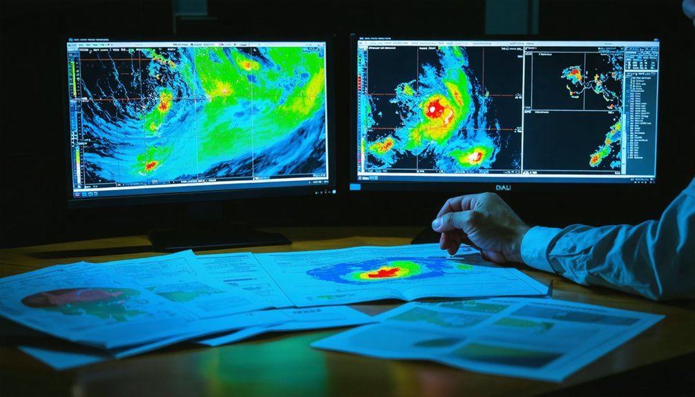
Radar and satellite data shift your analysis from potential to observed reality—they confirm whether the atmosphere is delivering what instability, moisture, and shear suggested it would.
Monitor satellite imagery through GOES loops to identify cloud-top cooling rates, overshooting tops, and mesoscale convective organization. These signals indicate updraft strength and system maturity before radar echoes fully develop.
Once convection initiates, switch your focus to radar loops to track cell motion, merger activity, and precipitation intensity. Measure storm movement vectors against your forecast trajectory to catch any deviation early.
Time-lapse radar loops reveal boundary interactions and discrete versus linear storm modes. Cross-reference both datasets continuously—satellite captures the broader convective environment while radar resolves internal storm structure, giving you an integrated, real-time picture of storm timing and movement.
Know What Triggers Severe Weather at the Local Level
Even when large-scale patterns look favorable, local triggers ultimately determine where and when severe weather fires. Surface convection doesn’t ignite randomly—specific boundaries and terrain features focus storm initiation.
Large-scale patterns set the stage, but local triggers decide exactly where and when severe weather strikes.
Monitor these four local triggers closely:
- Surface boundaries — Cold fronts, drylines, and outflow boundaries concentrate wind shear and moisture convergence into narrow initiation zones.
- Local topography—Terrain features force mechanical lift, channeling flow and accelerating surface convection along ridges, valleys, and slopes.
- Differential heating — Land-use contrasts between urban surfaces and rural areas create localized temperature gradients that destabilize the boundary layer.
- Sea and lake breezes — Coastal convergence zones generate focused lift that triggers convection independent of synoptic forcing.
Cross-reference surface observations with radar and satellite data to pinpoint exactly where initiation will occur.
Frequently Asked Questions
How Does Ocean Temperature Influence Storm Development and Intensity Forecasts?
Warmer sea surface temperatures fuel storm intensification by increasing evaporation and latent heat. You’ll track climate variability trends alongside SST anomalies to refine intensity forecasts, since elevated ocean heat content directly amplifies convective energy and precipitation potential.
What Role Does Soil Moisture Play in Convective Storm Initiation?
Like fertile ground feeding a flame, soil moisture fuels convective triggers by enhancing surface heat flux and boundary layer instability. You’ll find wetter soils amplify storm initiation potential, directly intensifying atmospheric lift and moisture availability overhead.
How Do Forecasters Communicate Storm Probability to the General Public?
You’ll find forecasters use probabilistic ensemble guidance to drive risk communication, translating model uncertainty into percentage-based outlooks. They issue tiered watches, warnings, and advisories that build public awareness by quantifying storm likelihood with precise, data-driven language.
Can Artificial Intelligence Improve Accuracy in Severe Weather Prediction Models?
Like a sharpened lens, machine learning refines your severe weather models—yes, AI can boost prediction accuracy. You’ll harness data integration across radar, satellites, and ensemble outputs, cutting RMSE and improving storm probability forecasts dramatically.
How Are Post-Storm Surveys Used to Improve Future Forecasting Methods?
You’ll use post-storm analysis to validate radar, model, and observational data against ground truth. It’s driving data calibration efforts that refine storm parameters, sharpen forecast algorithms, and strengthen your predictive accuracy for future severe weather events.
References
- https://www.ametsoc.org/ams/about-ams/ams-statements/statements-of-the-ams-in-force/weather-analysis-and-forecasting2/
- https://research.noaa.gov/three-ways-noaa-research-works-to-improve-our-weather-forecasts/
- https://www.cc-ema.org/post/severe-wx-forecasting-timelines
- https://crazystormchasers.com/temporal-analysis-of-meteorological-data-for-storm-forecasting/
- https://www.weather.gov/media/rah/NCStateStudents/handout.forecast.process.pdf
- https://www.weather.gov/media/zhu/ZHU_Training_Page/Met_Tutorials/Meteorological_Techniques.pdf
- https://www.youtube.com/watch?v=OXirhbRkgzs