To predict severe weather, you need to understand the air mass fueling it. Air masses are large bodies of air with uniform temperature and humidity, classified by origin — like cold, dry continental polar (cP) or warm, moist maritime tropical (mT). Their interactions create sharp gradients that destabilize the atmosphere. Key metrics like MLCAPE above 1,000 J/kg and storm-relative helicity above 150 m²/s² signal serious storm potential. There’s much more to unpack.
Key Takeaways
- Air masses are large bodies of uniform temperature and humidity that serve as fundamental building blocks shaping atmospheric stability and severe weather potential.
- Air masses are classified by origin: continental polar (cold, dry), maritime tropical (warm, moist), maritime polar, and continental tropical.
- Collisions between contrasting air masses, like continental polar and maritime tropical, create sharp gradients that destabilize the atmosphere and trigger severe weather.
- CAPE values above 2,500 J/kg combined with bulk shear exceeding 40 knots and helicity above 300 m²/s² signal high-confidence severe storm environments.
- Forecasters use NWP models, satellite imagery, rawinsonde balloon data, and isotach analysis to track air mass interactions and assess severe weather potential.
What Is an Air Mass and Why Does It Matter?
When you examine the atmosphere’s building blocks, air masses stand out as foundational elements for understanding severe weather. An air mass is a large body of air maintaining uniform temperature and humidity throughout its extent. You’ll find that air mass evolution directly shapes regional climate influence, determining whether conditions remain stable or deteriorate rapidly.
Air masses are the atmosphere’s building blocks—shaping severe weather and determining whether regional conditions stay stable or collapse.
Classification relies on two key variables: temperature origin (polar or tropical) and moisture source (maritime or continental). These designations—cP, mT, mP, cT—immediately communicate core atmospheric properties.
Polar source regions produce cold, dry air masses, while subtropical high-pressure belts generate warm, moist tropical masses.
Understanding these classifications gives you precise forecasting leverage. Temperature, pressure, and moisture profiles within each mass dictate stability, vertical motion potential, and ultimately, severe weather risk.
How Air Masses Are Classified by Source Region
Source regions define an air mass’s fundamental characteristics before it ever moves into your forecast area. You’ll classify each mass using two key variables: temperature origin (polar or tropical) and surface type (maritime or continental). These source region boundaries directly control moisture and thermal profiles you’ll analyze.
Continental polar (cP) air masses deliver cold, dry conditions from Canada’s interior. Maritime tropical (mT) air masses pull warm, moisture-laden air from the Gulf of Mexico. Maritime polar (mP) originates over cold ocean surfaces, while continental tropical (cT) develops over hot, arid land.
Air mass dynamics shift dramatically once a mass leaves its source region. Tracking that origin point lets you anticipate stability changes, dewpoint trends, and ultimately, your severe weather potential before you ever open a model output.
How Temperature and Moisture Define Air Mass Stability
When you analyze an air mass, temperature and moisture are your two primary stability indicators—temperature controls the lapse rate, while dewpoint measurements quantify available atmospheric moisture.
You’ll find that a stable air mass resists vertical motion, producing calm, stratiform conditions, whereas an unstable air mass accelerates convective currents upward, driving turbulence and severe weather potential.
As you track an air mass moving over a warmer surface, you’re watching instability build from below, a critical trigger you must account for in any severe weather forecast.
Temperature’s Role In Stability
Temperature and moisture work together to define an air mass’s stability profile, directly influencing whether severe weather develops. When you analyze air mass composition, temperature gradients become your primary diagnostic tool.
A steep temperature gradient—where surface temperatures markedly exceed upper-level temperatures—signals atmospheric instability, freeing vertical motion and triggering convective development.
You’ll measure stability using dewpoint and temperature readings at multiple atmospheric levels. When an air mass moves over a warmer surface, heat transfers upward from below, destabilizing the column and generating convective currents.
Conversely, a warmer upper atmosphere trapping cooler surface air creates stable conditions, suppressing vertical motion entirely.
Understanding these temperature-driven dynamics lets you accurately assess storm potential before committing to a severe weather forecast, giving you the analytical edge precision forecasting demands.
Moisture And Dewpoint Measurements
Moisture operates alongside temperature as the second half of your stability equation, and dewpoint measurements give you the quantitative handle you need on it. Dewpoint tells you the temperature at which air becomes saturated, triggering cloud formation and releasing latent heat that further destabilizes the atmosphere.
Higher dewpoints signal greater moisture transport into your target area, amplifying storm potential markedly.
You’ll track dewpoints as your primary moisture metric. Values above 60°F indicate adequate fuel; above 65°F, you’re entering high-octane territory.
When moisture transport from the Gulf streams northward, dewpoints spike rapidly, reshaping your stability profile within hours.
Cross-reference dewpoint data against MLCAPE values to quantify exactly how much atmospheric fuel your system can access before committing to a severe weather forecast.
Stable Versus Unstable Air
How an air mass behaves under forcing comes down to one core question: does it resist or encourage vertical motion? Stability is determined by temperature gradients between the air mass and the surface it’s traveling over.
When air mass origin is continental and polar, the air is typically stable—it resists lifting and produces little convective threat. But when that same air passes over warmer terrain, surface heating destabilizes it from below, generating convective currents.
You’ll assess instability using MLCAPE values. Readings above 1,000 J/kg signal meaningful atmospheric fuel. Unstable air facilitates the vertical motion storms need to intensify.
Track temperature gradients carefully—they’re your direct indicator of whether an air mass will suppress or accelerate severe weather development.
The Four Core Ingredients Every Severe Storm Needs From an Air Mass
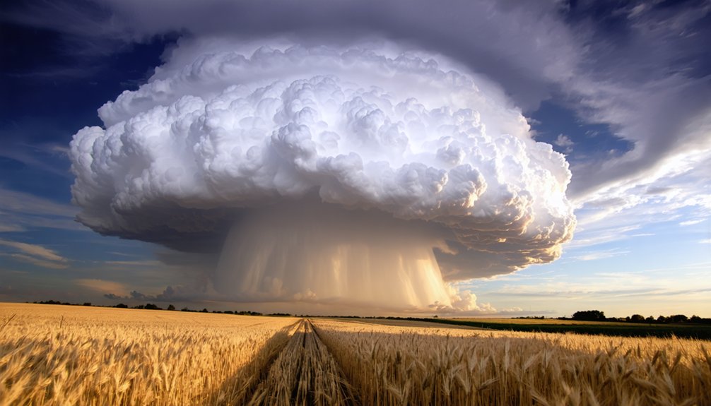
When forecasting severe weather, you’ll find that four core ingredients must converge within an air mass or along its boundaries: moisture, instability, lift, and wind shear.
Air mass origins directly dictate moisture availability, measured through dewpoints—your primary lifeblood metric for storm development.
Temperature effects determine instability, quantified using Mean Layer CAPE (MLCAPE), which reveals atmospheric fuel potential. Without sufficient CAPE, storms simply won’t sustain themselves.
Lift mechanisms—cold fronts, drylines, and terrain features—initiate convective development by forcing air upward.
Wind shear, particularly directional shear within the 0-6 kilometer layer, creates atmospheric spin that supercells ingest.
Helicity values exceeding 300 signal a very favorable severe weather environment.
When all four ingredients align simultaneously, you’re looking at significant severe weather potential requiring immediate action.
How Stable vs. Unstable Air Masses Determine Storm Potential
When you assess an air mass’s stability profile, you’re measuring its resistance to vertical motion using temperature and dewpoint data at multiple atmospheric levels.
If the air mass is stable, it suppresses convection and produces benign conditions.
If it’s unstable, it accelerates vertical motion, fueling the turbulence and convective currents that drive severe weather.
You can quantify that instability precisely using Mean Layer CAPE (MLCAPE), where higher values signal greater atmospheric fuel available for storm development.
Defining Atmospheric Stability Profiles
Whether an air mass produces calm skies or explosive thunderstorms hinges on its stability profile. You determine stability by analyzing temperature and dewpoint measurements through the atmospheric column.
When an air mass origins trace back to warm, moist regions within global circulation patterns, it often carries latent energy that fuels instability.
Stable air resists vertical motion, suppressing convection and producing stratiform clouds or fog. Unstable air accelerates vertical motion, driving convective currents that build severe thunderstorms.
The critical trigger is surface heating differential — when an air mass moves over a warmer surface, low-level warming destabilizes the column rapidly.
You’ll quantify instability using MLCAPE values. Higher CAPE directly correlates with increased severe weather potential, giving you precise, actionable data for accurate forecasting decisions.
Instability Fuels Severe Storms
Stability determines everything about storm potential — unstable air masses don’t just allow severe weather, they actively generate it. When you analyze air mass origin, you’re identifying the foundational temperature and moisture characteristics that dictate atmospheric behavior.
Continental polar air clashing against maritime tropical air creates sharp temperature gradients that destabilize the column rapidly.
You’ll quantify this instability using Mean Layer CAPE (MLCAPE). Values exceeding 2,500 J/kg signal serious atmospheric fuel, while values above 4,000 J/kg indicate explosive storm potential.
An air mass warmed from below loses its capping structure, triggering violent convective motion. You’re not guessing at that point — the data tells you exactly when unstable air transforms from passive atmospheric condition into an active severe weather engine demanding your immediate forecasting attention.
Measuring Convective Storm Potential
Quantifying convective storm potential requires translating raw atmospheric data into actionable thresholds you can apply directly to forecasting decisions. Air mass composition and source region analysis give you the foundation for interpreting these metrics accurately.
Use these four MLCAPE benchmarks to assess instability:
- 0–1,000 J/kg – Marginal instability; organized convection unlikely
- 1,000–2,500 J/kg – Moderate instability; supercell development possible with adequate shear
- 2,500–4,000 J/kg – Significant instability; violent storms probable
- 4,000+ J/kg – Extreme instability; life-threatening severe weather likely
Cross-reference MLCAPE against 0–6 km bulk shear values. When shear exceeds 40 knots alongside high CAPE, you’ve identified a high-confidence severe weather environment.
Don’t forecast in isolation—layer your metrics for precision.
How Fronts Trigger Severe Weather Between Competing Air Masses
When two contrasting air masses collide, fronts emerge as the battle lines where severe weather ignites. You’re watching air mass composition clash directly—cold, dry Canadian polar air driving southward against warm, moist Gulf moisture. Source region dynamics dictate each mass’s temperature and humidity profile, creating sharp gradients across frontal boundaries.
Cold fronts force warm air upward rapidly, generating instability and triggering convective development. The jet stream’s positioning amplifies this conflict, allowing polar surges to penetrate deep into warm sectors.
Wave cyclones form along these boundaries as low-pressure circulations exploit temperature contrasts.
Your forecasting advantage lies in identifying where helicity exceeds 150 m²/s², MLCAPE builds aggressively, and frontal lift converges. Those convergence zones are precisely where severe weather probability spikes highest.
How to Read Helicity Values and CAPE for Severe Weather Risk
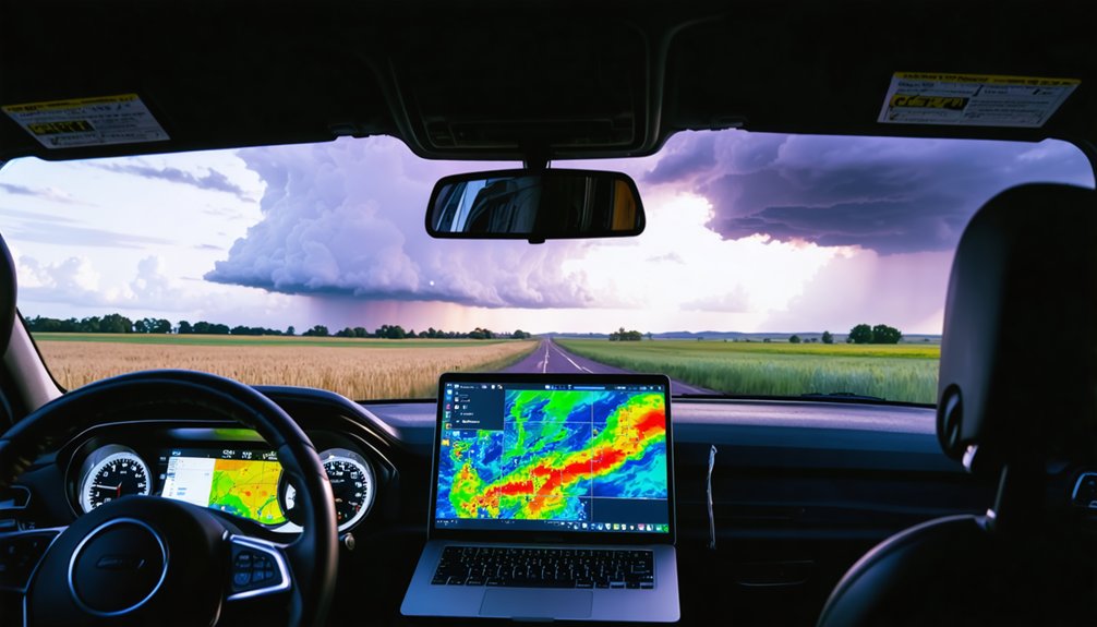
When you assess severe weather risk, you’ll rely on two core metrics: Mean Layer CAPE (MLCAPE) and 0–3 km storm-relative helicity (SRH).
You read CAPE as atmospheric fuel—higher values indicate greater instability and updraft potential—while SRH thresholds below 150 signal unfavorable conditions, 150–300 indicate favorable spin potential, and values exceeding 300 point to a highly volatile environment.
You sharpen your forecast by combining both metrics, since high CAPE with strong helicity dramatically increases the probability of supercell development and significant severe weather.
Understanding CAPE Values
Evaluating severe weather risk requires two critical atmospheric metrics: Convective Available Potential Energy (CAPE) and storm-relative helicity (SRH).
Air mass composition and source region dynamics directly influence CAPE readings, determining how much atmospheric fuel exists for storm development.
Use these MLCAPE thresholds to assess instability:
- 0–1,000 J/kg – Weak instability; minimal convective potential
- 1,000–2,500 J/kg – Moderate instability; organized storm development possible
- 2,500–3,500 J/kg – High instability; significant severe weather potential
- 3,500+ J/kg – Extreme instability; violent storm development likely
You’ll maximize forecast accuracy by cross-referencing CAPE values against SRH readings.
When MLCAPE exceeds 2,500 J/kg alongside SRH values above 300, you’re analyzing a genuinely dangerous atmospheric environment demanding immediate attention.
Interpreting Helicity Thresholds
Storm-relative helicity (SRH) completes the severe weather picture that CAPE values begin to paint. When you’re analyzing helicity thresholds, three distinct ranges define your risk assessment.
Values below 150 J/kg signal an unfavorable environment — storms won’t organize efficiently.
Between 150 and 300 J/kg, you’re entering favorable territory where wind shear begins generating meaningful atmospheric rotation.
Above 300 J/kg, you’ve identified a genuinely dangerous setup where supercell development becomes highly probable.
Wind shear direction matters as much as magnitude. You need to combine SRH readings with your MLCAPE values to build a complete picture.
High CAPE paired with strong helicity thresholds creates compounding risk.
Position yourself east of a dryline, south of a cold front, and these metrics sharpen dramatically — that’s your highest-probability severe weather corridor.
Combining Metrics For Forecasting
Reading helicity and CAPE in isolation gives you an incomplete forecast — you need both metrics working together to accurately assess severe weather risk.
Air mass composition and source region dynamics directly influence both values, so cross-referencing them sharpens your risk assessment.
Follow this decision framework:
- Confirm MLCAPE exceeds 1,000 J/kg — sufficient atmospheric fuel exists for storm development.
- Verify 0-3 km helicity surpasses 150 m²/s² — rotational potential becomes meaningful.
- Check helicity exceeds 300 m²/s² — supercell probability increases considerably.
- Position yourself east of the dryline, south of the cold front — boundary overlap maximizes storm initiation.
When CAPE and helicity both hit critical thresholds simultaneously, your severe weather probability escalates markedly. Neither metric alone tells the complete story.
How Forecast Models Analyze Air Mass Behavior in Real Time

To analyze air mass behavior in real time, forecasters rely on Numerical Weather Prediction (NWP) models that ingest atmospheric data from radiosondes, satellites, and surface observations into supercomputers running complex mathematical equations.
These models track air mass interactions by monitoring temperature gradients, moisture flux, and stability indices across multiple atmospheric layers.
You’ll want to pay close attention to surface temperature differentials, as they reveal where contrasting air masses converge and intensify frontal boundaries.
Models also integrate isotachs to pinpoint jet stream positioning, which directly influences polar air surges southward.
Which Satellite and Upper-Air Tools Track Air Mass Movement
Satellite and upper-air tools give you the observational backbone for tracking air mass movement with precision. Satellite imagery reveals air mass boundaries, moisture gradients, and cloud structure in real time. Upper air analysis through rawinsonde balloon data captures temperature, dewpoint, and wind profiles at multiple atmospheric levels.
Together, they let you pinpoint where contrasting air masses collide and instability builds.
Here are four essential tools you’ll rely on:
- Visible and infrared satellite imagery — identifies air mass boundaries and cloud patterns
- Water vapor imagery — tracks moisture transport and upper-level dynamics
- Rawinsonde soundings — measures vertical temperature and dewpoint profiles
- Isotach analysis — locates jet stream positioning and maximum wind speed corridors
These tools give you independent observational leverage no model alone provides.
How Meteorologists Build a Severe Weather Forecast From Air Mass Data
Once you’ve gathered observational data from satellite imagery and upper-air soundings, the real analytical work begins—synthesizing that raw information into an actionable severe weather forecast. You’ll assess air mass origins first—whether continental polar or maritime tropical—because temperature effects directly determine instability potential. Plot dewpoints to gauge moisture, then calculate MLCAPE to quantify atmospheric fuel.
Check 0-6 kilometer bulk shear and 0-3 kilometer helicity; values exceeding 300 signal a highly favorable severe weather environment. Identify your lift mechanisms—cold fronts, drylines, or terrain. Position matters: being east of a dryline and south of a cold front maximizes storm probability.
Feed this data into NWP models, cross-reference with isotach analysis to locate the jet stream, and you’ve built a precise, data-driven severe weather forecast.
Frequently Asked Questions
Can Air Masses Influence Air Quality and Pollution Dispersal Patterns?
Yes, air masses directly control urban pollution dispersal through air circulation patterns. Stable air traps pollutants near the surface, while unstable air disperses them vertically. You’ll notice worse air quality when stagnant high-pressure systems dominate your region.
How Long Does a Typical Air Mass Retain Its Original Source Region Properties?
Remarkably, you’ll find air masses retain source region stability for 3–5 days before modification. Temperature retention weakens as they traverse contrasting surfaces, with properties shifting roughly 20% per 500km of travel over differing terrain.
Do Air Masses Behave Differently Over Mountainous Terrain Versus Flat Plains?
Yes, they do! Over mountainous terrain, you’ll notice mountainic influence forces air upward, triggering instability. On flat plains, plains stability dominates, allowing air masses to retain properties longer, making severe weather forecasting more predictable.
Can Two Air Masses of the Same Classification Ever Merge Together Completely?
Merging’s nearly impossible! Even identical classifications retain distinct air mass boundaries due to subtle temperature and dewpoint differences. You’ll find classification overlaps exist, but complete fusion never truly occurs in measurable atmospheric data.
How Do Air Masses Affect Marine Weather Conditions and Coastal Fishing Safety?
When air mass interactions shift coastal weather patterns, you’ll face rapid wind changes, fog, and dangerous swells. Monitor dewpoints, stability profiles, and frontal boundaries to protect your vessel and optimize your fishing safety decisions.
References
- https://www.noaa.gov/education/resource-collections/weather-atmosphere/weather-systems-patterns
- https://geo.libretexts.org/Bookshelves/Geography_(Physical)/Introduction_to_Geography_(McCormick)/01:_Physical_Geography/1.06:_Atmosphere-_Air_Masses_and_Storms
- https://www.weather.gov/okx/WinterWeatherAwareness
- https://www.youtube.com/watch?v=1Nok6NDoHN0
- https://www.aopa.org/training-and-safety/online-learning/safety-spotlights/weather-wise-air-masses-and-fronts/air-masses
- https://crazystormchasers.com/analyzing-air-masses-for-severe-weather-forecasting/
- https://www.faa.gov/regulations_policies/handbooks_manuals/aviation/Balloon_Flying_Handbook_FAA-H-8083-11B/bfh_chapter_4.pdf
- https://www.faasafety.gov/files/events/SO/SO15/2024/SO15129440/FAA-H-8083-28-Chpt11.pdf
- https://www.metoffice.gov.uk/binaries/content/assets/metofficegovuk/pdf/research/library-and-archive/library/publications/factsheets/factsheet_10-air-masses-and-weather-fronts_2023.pdf